Chapter 2: Tera Calculation 0 - Shipping Data Processing
Section 0: Flow of Tera Calculation 0
Based on the reference materials, we will explain the role and processing flow of "Tera Calculation 0", which is the first stage of shipping data analysis.
Role of Tera Calculation 0
Tera Calculation 0 is a software tool used to organize and process raw shipping data into an easily manageable format prior to calculating the scale of the distribution center (Tera Calculations 1 & 2). At this stage, frequently calculated common data is created and stored in advance as the "T200" table in Access.
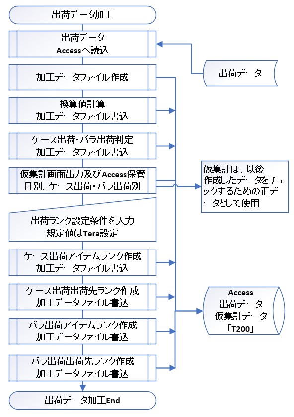
4 Steps of Processing
Specifically, the data is processed through the following steps:
- Separation of Shipping Forms: Shipping data is divided into "Case Shipping" and "Piece Shipping".
- Unit Conversion: Piece count data is converted in bulk into "Case Count," "Pallet (PL) Count," "Volume," and "Weight," which are essential for logistics design.
- Creation of Ranks: Data is aggregated by shipping destination and item (product), and "Destination Ranks" and "Item Ranks" are assigned based on their respective liquidity.
- Generation of the "T200" Table: The data table that forms the core of the analysis, integrating all the above information, is finalized.
Importance of Grouping by Liquidity
To design an efficient distribution center, it is crucial to accurately group items into high-liquidity and low-liquidity categories and allocate appropriate equipment and operations to each.
- The 80:20 Rule (Pareto Principle): In the past, it was said that "20% of items account for 80% of the volume." Today, due to improved information management accuracy, the trend is roughly 20% of items accounting for 50% of the volume, and 30% of items accounting for 65–70%.
- Aim of Tera Calculation 0: By clearly distinguishing these liquidity differences, the optimal layout for equipment and facilities can be derived.
Section 1: Contents of Shipping Data
This material explains the "Contents of Shipping Data" and the "Concept of Shipping Fluctuations", which serve as the foundation for distribution center design.
1. Components of Shipping Data (EIQ + α)
The basis of logistics design is EIQ Analysis (Entry: Destination, Item: Product, Quantity: Amount). However, for highly accurate design, Tera Calculation adopts a data format with the following added items:
Basic EIQ Items
- Destination (E): The company or store name where products are delivered.
- Item (I): The product name or code distinguishable at the SKU (Stock Keeping Unit) level.
- Piece Count (Q): The minimum unit for management and operations.
Additional Items for Logistics Design
- Shipping Date & Time: Used for calculating hourly volume and analyzing the "fluctuations" described below.
- Item Category & Shipping Category: Used for extracting or excluding specific ranges of products/destinations.
- Shipping Route: Used to manage groups loaded onto the same truck.
- Conversion Data: "Items per Case," "Cases per PL," "Case Volume/Weight," etc. These are used to convert the piece count into logistical units (cases, pallets, volume).
2. Shipping Fluctuations and Economical Scale Design
Shipping volume is not constant every day; it fluctuates by season, month, day of the week, and even due to weather or new store openings. This is called "Shipping Fluctuations".
Strategies for an "Economical Scale" Distribution Center
If a facility is built to handle the absolute peak (the crest of shipping fluctuations), it will result in vast wasted space during the off-season, which is uneconomical. Tera Calculation presents the idea of deliberately selecting a non-peak day (e.g., a Thursday rather than the weekly maximum) as the target day.
- Measures During Peak Times: Instead of over-scaling the facility, peaks are managed through the following operational strategies:
- Extending operating hours or increasing the number of workers.
- Outsourcing to other facilities or front-loading shipping tasks.
- Company-wide Consensus: Since these measures affect purchasing and sales departments as well, building consensus across departments is crucial.
3. Scale of Analysis Data
In the example shown in the materials (assuming a BtoB center for small home appliances and electronic devices), the data scale is as follows:
- Number of Records: 60,000 rows.
- Positioning: Corresponds to the upper end of mid-scale or the lower end of large-scale operations.
Item 1: Shipping Data Items
A distribution center ships products based on orders from destinations. A compilation of these shipping records is called shipping data.
It is a record of E (Entry), I (Item), and Q (Quantity), meaning "Shipped 10 units of Product B to Destination A."
In Tera Calculation, designing a distribution center is impossible using only the EIQ information mentioned above, so necessary items have been added.
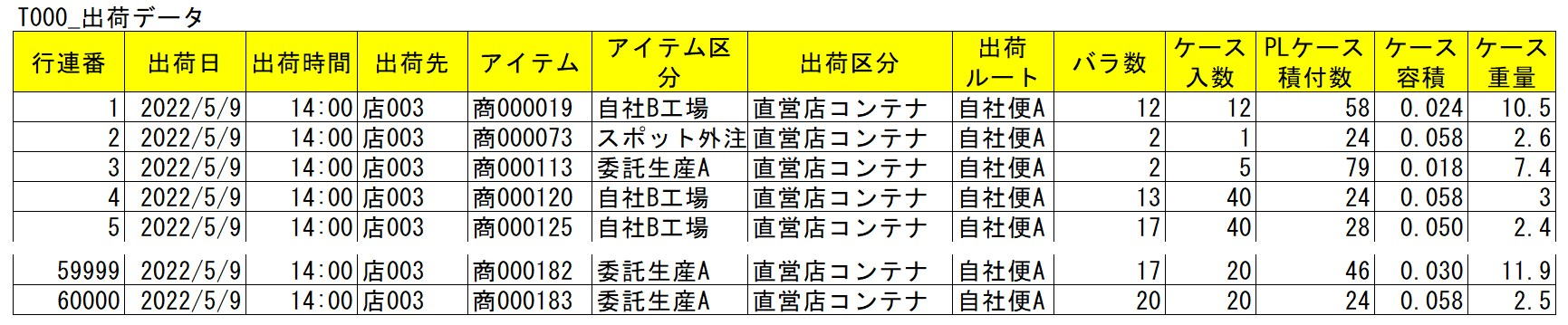
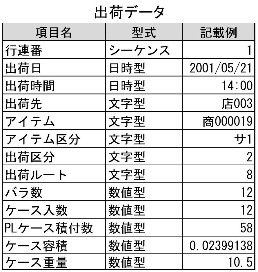
Row Number: The order sequence of the shipping data record (a sequential number assigned to the record).
Shipping Date: The date shipped (shipping data contains multiple dates).
Shipping Time: The time shipped, used for hourly volume aggregation.
Destination (E): The company or store name where the product is delivered.
Item (I): Product name or code (must be distinguishable by SKU).
Item Category: Used to extract or exclude an item range during aggregation. Enter "None" if unnecessary.
Shipping Category: Used to extract or exclude a destination range during aggregation. Enter "None" if unnecessary.
Shipping Route: The shipping route name for a group of destinations loaded on the same truck, or a route name to manage grouped destinations.
Piece Count (Q): The minimum unit for operations and management (SKU).
SKU (Stock Keeping Unit) is the smallest management unit for ordering and inventory control, used to distinguish items by factors like case quantity or product size.
Items per Case: Used to calculate case conversion and distinguish between case shipping and piece shipping.
Cases per PL: Used to calculate pallet conversion (hereafter called PL Conversion); the number of cases that can be stacked in a specified pallet configuration.
Case Volume: An item for converting piece counts into volume (calculated after case conversion).
Case Weight: An item for converting piece counts into weight (calculated after case conversion).
The shipping data used in Tera Calculation (see attached Excel) does not allow changes to data item columns or item names. Please understand this as a rule when importing shipping data into Tera Calculation.
Simple Aggregation of Shipping Data
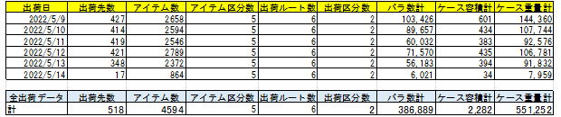
Shipping data consists of 60,000 records.
The scale of the distribution center is positioned around the upper mid-scale to lower large-scale.
The industry assumed is a BtoB-focused distribution center primarily handling small home appliances and electronic devices.
Item 2: About Shipping Data Fluctuations
Shipping volume increases and decreases daily. Plotting this on a daily graph creates a wave-like curve, which is called shipping fluctuation.
A company's sales fluctuate by season, month, and day of the week, and shipping volume correlates with sales. It is also necessary to consider that product volumes may differ by season (summer vs. winter goods) depending on the industry.
Building a distribution center to match these peak shipping data fluctuations results in an oversized facility and is uneconomical.
To design an economically scaled distribution center, we verify the difference between the shipping data adopted for calculations and the peak shipping days, as well as what countermeasures can be taken during peak times.
Countermeasures include extending working hours, increasing staff, delegating to other facilities, and front-loading shipping tasks (operational changes). These measures impact not only logistics but also purchasing and sales departments, so it is necessary to explain them and obtain company-wide consensus.
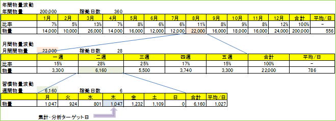
The above table is a volume fluctuation table created to determine the target day for aggregation and analysis, formulating a distribution center tailored to August volumes.
The intent behind selecting Thursday—which is not the weekly maximum—as the target day is to manage peak days via extended hours, staff increases, or outsourcing, thereby maintaining the distribution center at an economical scale.
Logistics fluctuations occur not only by year, month, or week, but also due to public holidays, weather, and the opening of new customer stores.
Section 2: Shipping Data Processing
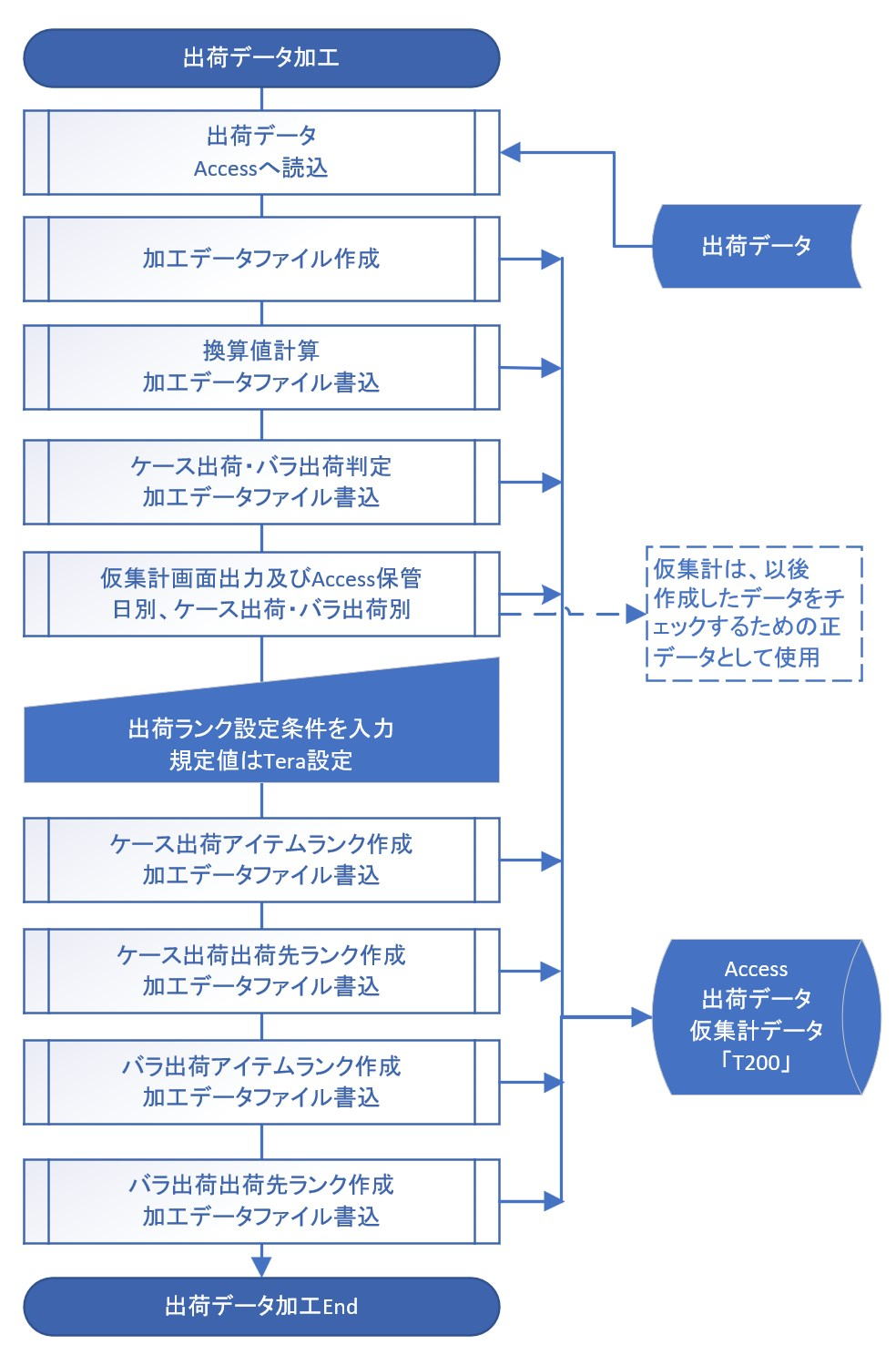
This material explains the specific procedures and calculation logic for "Shipping Data Processing (Tera Calculation 0)", the cornerstone of shipping data analysis.
1. Data Import and Basic Conversion
First, shipping data in Excel format is imported into Access to create the "T000_ShippingData" table.
Immediately after import, the following conversion values—essential for logistics design—are calculated for each record (row):
- Case Conversion: Piece Count ÷ Items per Case
- PL Conversion: Case Conversion ÷ Cases per PL
- Volume/Weight Conversion: Case Conversion × Case Volume (or Weight)
2. Separation of Case Shipping and Piece Shipping
Because storage locations and operational methods differ between case units and piece units in a distribution center, these are clearly separated for aggregation.
- Case Shipping: Orders of 1 whole case or more. Products are retrieved from the inventory area and transported directly to the sorting area.
- Piece Shipping: Orders of less than 1 case, or fractional orders. Products are picked from shelves in the shipping operation area.
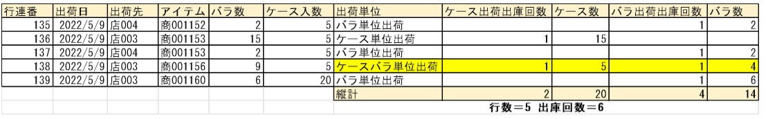
- Example: For an order of 9 units of a product packaged in 5 units per case, it is separated and counted as 1 Case (Case Shipping) and 4 Pieces (Piece Shipping).
3. 5-Level Ranking (Extension of EIQ Analysis)
A detailed 5-level ranking—more granular than general ABC analysis (3 categories)—is performed to optimize equipment allocation and operations.
- Rank Ratios (Tera Settings): A1 (50%), A2 (20%), B (15%), C (10%), D (5%).
- Ranking Keys:
- Tera Calculation 1: Ranks are based on "Case Conversion" for case shipping, and "Row Count (Retrieval Frequency)" for piece shipping.
- Tera Calculation 2: Since the primary purpose is calculating storage volume, both use "PL Conversion" as the standard.
4. Creation of the "T200" Table
A single integrated table named "T200" is created, containing all processed data (conversion values, shipping categories, and rank information). Tera Calculations 1 and 2 achieve faster processing speeds by referring exclusively to this table.
5. Definition of Terms and Operational Supplements
- Definition of Retrieval Frequency: If both cases and pieces are shipped in a single record, Tera Calculation counts this as "Retrieval Frequency: 2" to accurately capture the actual workload.
- Storage / Retrieval: Receiving items into and taking items out of storage space.
- Sorting / Picking: Distributing retrieved products is defined as "Sorting (Seeding)," while gathering products from operational shelves is defined as "Picking."
- Consideration of Time Zones: The peak of each process is calculated backward based on the shipping time. Note that upstream processes (like picking) must start and finish earlier.
Item 1: Shipping Data Import
Bringing data into Access is called importing, and taking data out of Access is called exporting.
In "Tera Calculation 0", taking Excel shipping data into Access and creating the "T000_ShippingData" table is referred to as importing shipping data.
Access is initialized (cleared) before importing, so at the time of import, only the "T000_ShippingData" table exists in Access.
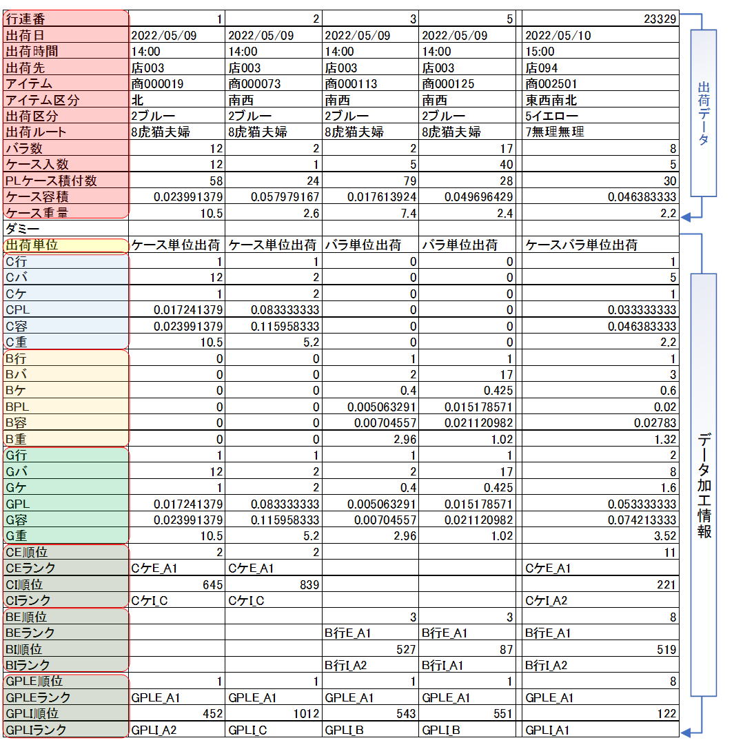
Item 2: Calculating Each Conversion Value from Piece Count
The first process performed by the Tera Calculation 0 Data Processing Software is calculating conversion values for cases, PLs, volume, and weight, which are not present in the original shipping data.
The formulas are:
Case Conversion = Piece Count / Items per Case
PL Conversion = Case Conversion / Cases per PL
Volume Conversion = Case Conversion * Case Volume
Weight Conversion = Case Conversion * Case Weight
Conversion values are recorded on a per-record basis.
Item 3: Classifying Case Shipping and Piece Shipping
Distribution centers handle cargo operations in units of PLs, cases, and pieces.
Tera Calculation separately analyzes and aggregates case unit shipping and piece unit shipping. This is because work processes and storage methods differ for each.
Calculations:
1. Less than 1 case is piece shipping (Case Conversion < 1).
2. If 1 case or more and there are no decimals (e.g., 1.0, 5.0), it is case shipping (Case Conversion >= 1 and Piece Count mod Items per Case = 0).
3. If 1 case or more and there are decimals (e.g., 1.1, 5.3), it is a mixed case/piece shipping (Case Conversion > 1 and Piece Count mod Items per Case <> 0).
4. In the case of 3, the integer part becomes case shipping, and the decimal part becomes piece shipping.
Case Count for Case Shipping = Int(Piece Count / Items per Case)
Piece Count for Piece Shipping = Piece Count - (Case Count * Items per Case)
Calculation Example:
When shipping 9 pieces of Product B (which has 5 items per case) to Destination A, it is shipped as 1 case and 4 pieces.
For operations, the 1 case is batch-retrieved from the inventory area alongside identical items for other destinations and sorted in the sorting area.
The 4 pieces are picked and retrieved from flow racks or medium-duty shelves in the shipping operation area.
The classification of case shipping and piece shipping is calculated on a per-record basis.
Calculations in PL units can be derived as needed from the conversion values.
Note: In small-scale centers, case shipping (e.g., 2 cases) and piece shipping (e.g., 3 pieces) might be retrieved simultaneously from the inventory area, but Tera Calculation assumes a center where case and piece shipping operations are clearly separated.
These calculation results are saved in the "T110_CategoryConversion" table.

In the table above, "C row" means the number of rows for case shipping, "B row" means the number of rows for piece shipping, and "G row" means the number of rows for case + piece shipping combined.
The first character (C, B, G) indicates the shipping category. The subsequent characters mean: row = row count, p = piece count, c = case conversion, pl = pallet conversion, v = volume conversion, w = weight conversion.
Item 4: Assigning Ranks
Assigning Ranks to Items
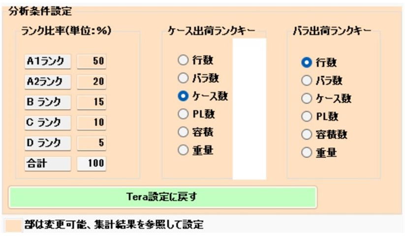
Ranking ratios are segmented into: A1 Rank (50%), A2 Rank (20%), B Rank (15%), C Rank (10%), and D Rank (5%).
These rank ratios can be modified, provided they total 100%.
Tera Calculation aggregates all shipping data by item and assigns sequential numbers and ranks from the highest liquidity item downward. This method is the same as ABC analysis. While ABC analysis generally uses 3 segments, Tera Calculation uses 5 segments. This is because having more rank segments makes it easier to construct distribution center operational rules and equipment setups.
From experience, 10 segments are too many, while 5 segments feel just right.
The item used for ranking can be "Record Count (Row Count)", "Piece Count", "Case Conversion", "PL Conversion", "Volume Conversion", or "Weight Conversion." Choosing which to use is open to debate.
Under Tera Settings, Tera Calculation 1 uses "Case Conversion" for case shipping and "Row Count" for piece shipping. Tera Calculation 2 uses "PL Conversion" for both.
While using Tera Calculation software to compare various ranking keys, there was no drastic difference in aggregation results that would make any specific setting definitively "wrong."
Assigning Ranks to Destinations
Destination ranking uses the same 5 segments as item ranking.
Destination ranking uses the same ratio settings as item ranking (Tera Settings).
Ratios and ranking keys can be modified.
Creating the "T200" Table by Linking "T180" and "T110" to "Shipping Data"
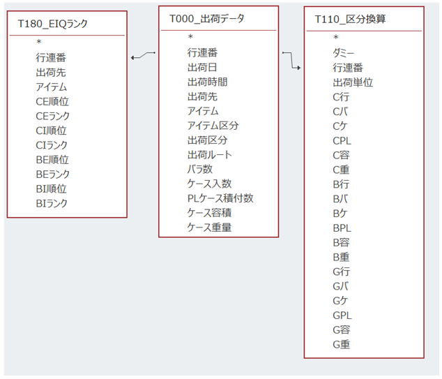
After creating the aforementioned "T110_CategoryConversion" and "T180_EIQ Rank" tables, they are joined with "T000_ShippingData" to create the new "T200" table.
The reason for using the "T200" table instead of standard table links is software convenience: SQL statement creation becomes simpler and processing speeds are improved.
Tera Calculations 1 & 2 access only the "T200" table to perform their analyses.
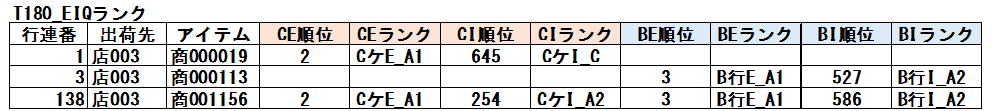
Item 5: Table File Layout
Items from "Row Number" to "Case Weight" reflect the original shipping data.
The "Dummy" field is set to Null and is used by Tera Calculation to insert calculation categories during processing. ("Unit" and subsequent fields contain data created by Tera Calculation 0).
In "C Row," C stands for the case shipping group, B for piece shipping, and G for combined case and piece shipping.
For ranking information, fields from "CE Order" to "CI Rank" relate to case shipping, while "BE Order" to "CI Rank" relate to piece shipping (used in Tera Calculation 1). "GPL_E Order" to "GPL_I Rank" are ranking fields used in Tera Calculation 2.
Row 23329 shows a "G Row" value of 2, indicating that retrieval operations occurred twice (once for case and once for piece).
Ranking Keys
The ranking key is the numerical baseline used to determine ranks (data is aggregated by this key to assign ranks).
If Piece Count is the key, data is aggregated and ranked by piece quantity.
If Case Count is the key, data is aggregated and ranked by case conversion.
Tera Calculation 1 targets peak shipping days and uses "Row Count" for piece shipping and "Case Conversion" for case shipping as the ranking keys. This is used to calculate the output capability from inventory to the shipping operations area.
Tera Calculation 2 targets the all-data average and uses "PL Conversion" for both piece and case shipping. Distribution center scale calculations primarily involve storage capacity calculations, making PL and volume conversions more relevant.
Observations
In Tera Calculation 2 (Center Scale Calculation), you can change ratios or ranking keys and instantly see the change in distribution center area (results display in 1-2 minutes).
Separating ranking between case shipping and piece shipping is necessary because their operational methods completely differ.
If case and piece shipping are not separated, aggregating by retrieval frequency causes piece shipping to dominate the upper ranks, while aggregating by case conversion causes case shipping to dominate, creating contradictions.
Therefore, Tera Calculation selects the method of separating and analyzing piece and case shipping according to their specific contexts.
However, for inventory calculations, taking the average of all shipping data (piece + case) was deemed most rational.
While standard ABC analysis divides logistics into 3 ranks (A: 70%, B: 20%, C: 10%), 3 ranks often feel insufficient.
From experience, 5 rank segments allow for a balanced division of equipment allocation and operational categories.
Specific Steps for Ranking
Example: Item ranking for case shipping
1. Specify the item ranking key.
The ranking key is the field used for volume comparison (e.g., Shipping Frequency, Piece Count, Case Conversion, PL Conversion, Volume, Weight).
Tera Settings selects Case Conversion for case shipping, and Shipping Frequency for piece shipping.
2. Allocate the volume ratio to each rank.
Tera Settings divides this into 5 stages: A1 (50%), A2 (20%), B (15%), C (10%), D (5%).
3. Aggregate all records by item for case shipping.
Sort item aggregations in descending order of volume, and assign a sequential rank order.
Calculate cumulative volume and cumulative volume ratio based on the order, and assign a rank based on the ratios specified in step 2.
Link this item order and rank back to each record in the shipping data.
4. Calculate destination rank for case shipping. The calculation method is the same as 3.
5. Calculate item rank and destination rank for piece shipping. The calculation method is the same as 3.
6. Refer to the "T180_EIQ Rank" table for each rank category.
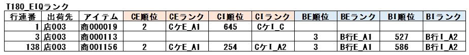
T180_EIQ Rank is the Access table name, CE Order means the destination order for case shipping, and CI Rank means the item rank for case shipping.
Item 6: Supplements Regarding Shipping Data
Generally, it is calculated as Record Count = Retrieval Frequency, but Tera Calculation treats Record Count and Retrieval Frequency as different units.
Record Count means the row of the shipping data, while Retrieval Frequency means the number of retrieval actions performed.
If 1 case and 3 pieces are shipped within 1 record, there is 1 retrieval operation for case shipping and 1 for piece shipping. Tera Calculation counts this as Record Count 1, but Retrieval Frequency 2.
Normally, placing a product on a shelf is called storage (Nyuko), and taking it out is called retrieval (Shukko). This results in using the exact same words for actions occurring in both the storage space and the operational space.
To avoid this overlap, this text expresses placing items into the storage space as "Kurayire" (Storage/Putaway), and taking items out of the storage space as "Kuradashi" (Retrieval).
Distributing retrieved products by destination is called Sorting (Seeding). Placing retrieved products onto shelves in the shipping operation area (replenishment) and taking them out from those shelves by destination (picking) is called Picking.
The word "Sorting" is often used to include both Seeding and Picking. Hereafter, please understand Sorting = Seeding, Picking = Picking, and General Sorting = Seeding + Picking.
Tera Calculation deals strictly with distribution center systems and does not touch upon transportation/delivery after loading onto a truck. Please refer to other materials for information on transportation.
All shipping data analysis aggregate figures use double precision (the highest accuracy on a PC). However, since calculation results go through multiple processing stages, minor errors cannot be denied. (Currently, no significant error displays have been confirmed). The screen display rounds off to integers as much as possible for readability, but the software retains double precision.
Distribution centers must possess the capacity to handle operations during peak time slots; if they cannot, countermeasures are necessary. This includes front-loading tasks or increasing staff. Please review the peak time aggregation in Tera Calculation while keeping these potential countermeasures in mind.

The peak time slot for each process is determined based on the shipping time in the shipping data, and shipping must be completed by that designated time. Therefore, note that the start and end times of upstream shipping processes will be shifted forward.
Dedicated Flights (In-house Fleet) vs. Courier Services
Dedicated flights (in-house fleet) are delivery systems where the shipper or logistics provider secures a dedicated delivery route and trucks strictly for the shipper.
Courier services are delivery systems where the shipping company secures its own fixed delivery routes and trucks, and the shipper requests delivery on a case-by-case basis.