Chapter 3: Tera Calculation 1_Shipping Data Analysis

Section 1: EIQ Matrix Calculation

This section explains the "EIQ Matrix Calculation (Analytical Aggregation)", which is the core of shipping data analysis.

1. Differences Between Conventional Calculation and EIQ Matrix Calculation

There are decisive differences between conventional logistics analysis (such as ABC analysis) and the EIQ Matrix Analysis proposed by Tera Calculation.

• Conventional Calculation (ABC Analysis): Because item aggregation and shipping destination aggregation are performed separately, the correlation between them is unknown. It is impossible to grasp "which rank of products flows to which rank of shipping destinations."
• EIQ Matrix Calculation (Tera Calculation): Aggregates data by linking them into 25 blocks: "Item Rank (5 categories) × Shipping Destination Rank (5 categories)". This makes it possible to accurately grasp the physical volume flowing from a specific item rank (equipment) to a specific shipping destination rank (shipping area).

2. What Can Be Read from the EIQ Matrix Table

Utilizing this table makes it easier to study specific specifications for a distribution center.

• Grasping Workload: You can check the picking frequency, total piece quantity, volume, and weight by rank.
• Equipment Optimization: You can calculate the number of items that require flow racks, or the number of cases and pallets needed for replenishment on a block-by-block basis.
• Flexibility in Conversion Units: All numerical values are converted from the piece quantity, and the display can be toggled between units such as cases, PL (pallets), volume, and weight.

3. How to Read Rank Symbols

To prevent confusion, rules are established so that the target of aggregation can be identified at a glance.

4. Analysis Operation Procedure

On the Tera Calculation 1 screen, analysis is processed using the following procedure.

1. Select Characteristics: Select the target day by specifying a shipping date or choosing characteristics such as "Maximum Case Shipping Day."
2. Specify Category and Unit: Select Case/Piece, Real Number/Ratio, and the Display Unit (Pieces, Volume, etc.).
3. Condition Extraction: Narrow down the target data using checkboxes for item categories, shipping categories, etc.
4. Execute: Click the Start button to output the results to the data grid view (table).

Observations and Points to Note

• Visualization: Large-scale data (over 400 destinations, over 4000 items) cannot be fully grasped with a standard EIQ table. Grouping it using a Matrix Table or an EIQ Scatter Plot (to visually grasp dispersion) is highly effective.
• Recording Details: When cropping the table to create documents, be sure to note the "Shipping Method", "Shipping Date", and "Display Unit" alongside it to prevent confusion later.

---

Item 1: Differences Between Conventional Calculation and EIQ Matrix Calculation

In Tera Calculation, calculations aggregated using the ABC analysis method are referred to as conventional calculations. While ABC analysis divides ranks into 3 categories and aggregates items and shipping destinations separately, Tera Calculation divides ranks into 5 categories and aggregates them.

In conventional calculation, although the totals for each item in the item aggregation and shipping destination aggregation are the same, there is no correlation between the two tables. Therefore, with conventional calculation, you cannot tell from these two tables how products in item rank A1 are distributed among the shipping destination ranks. When evaluating distribution center scales, operational methods, or calculating the physical volume of each process, data correlating shipping destinations and items is necessary.

Tera Calculation proposes a method of aggregating by dividing into 25 blocks (Item Rank 5 * Shipping Destination Rank 5 = 25 blocks), linking item ranks and shipping destination ranks. In Tera Calculation, this aggregation table is called the EIQ Matrix Table. Furthermore, Tera Calculation can display the number of rows (picking frequency), piece quantity, case conversion, PL conversion, volume conversion, and weight conversion within the same rank divisions.

With this EIQ Matrix Table, you can easily read off, for example, how many times item A1 rank products are picked from the flow racks in the shipping operation area, what the total piece quantity is, what the volume is at that time, how many shipping containers are needed, how many cases are needed to replenish the flow racks from the storage area, and how many pallets it equates to when transported from the storage area via mixed-load PLs.

The display units in the EIQ Matrix Table mean: "Piece" is piece quantity, "Case" is case conversion, "PL" is PL conversion, "Volume" is volume conversion, and "Weight" is weight conversion. Please note that hereafter, all physical volume units other than piece quantity are conversion units derived from the piece quantity (if the term "Case" is used, it implies "Case Conversion").

As mentioned earlier, the EIQ Matrix Table is an aggregation table divided into 5 * 5 = 25 blocks. The horizontal total is the aggregation of shipping destination volumes, and the vertical total is the aggregation of item volumes. If the display unit of the EIQ Matrix Table is set to PL conversion, the horizontal total matches the PL conversion of the conventional item aggregation, and the vertical total matches the PL conversion of the conventional shipping destination aggregation. Matrix aggregation and conventional calculation are linked and always display the same content. The same applies to the number of shipping destinations and items.

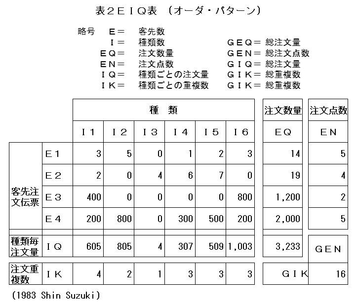
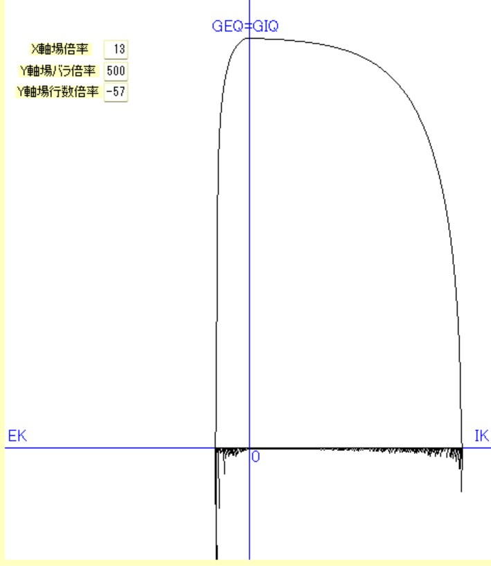
Differences Between the EIQ Table and EIQ Matrix Table

Fundamentally, designing a system by looking at the physical volume of which items go to which shipping destinations is the standard approach, and Mr. Shin Suzuki introduced this as the EIQ Table. Certainly, if there are about 50 shipping destinations and 100 items, it is possible to create and study an EIQ Table. However, with shipping data like the one used here, featuring over 400 destinations and over 4000 items, an EIQ Table would become a chart that cannot even fit in an 8-tatami room, making it impossible to fully read.

In Tera Calculation, we devised an aggregation method that groups the EIQ Table by ranks, and we decided to call this the EIQ Matrix Table.

Additionally, there is a method of displaying the EIQ Table as points to create a scatter plot. For 400 destinations and 4000 items, charting it allows you to horizontally scroll on a PC screen and visually observe the dispersion of the EIQ Table. In Tera Calculation, we decided to call this diagram the EIQ Scatter Plot (refer to Tera Calculation 4_Reference EIQ).

Next, we introduce the EIQ Graph devised by Mr. Shin Suzuki. This graph expresses a single day's physical volume in one diagram, using curves for the cumulative volume of shipping destinations and items, and bar graphs for the picking frequency of shipping destinations and items (refer to Tera Calculation 4_Reference EIQ).

Please refer to other publications for further details on the EIQ Table and EIQ Graph.

Item 2: Relationship Between Conventional Calculation and EIQ Matrix Calculation

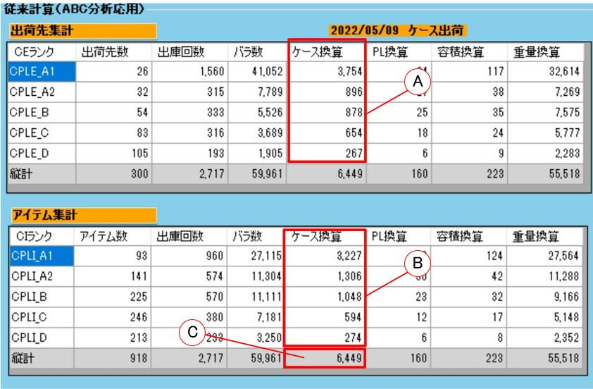
Since conventional calculation aggregates shipping destinations and items separately, the relationship between them remains unknown.

With EIQ Matrix aggregation, the physical volume of item rank A1 bound for shipping destination rank A1 is known, meaning the volume is aggregated with a correlation between shipping destinations and items.

Observation: With this EIQ Matrix Table, it is possible to grasp how much physical volume flows from each item rank (equipment) to each shipping destination rank (shipping area).

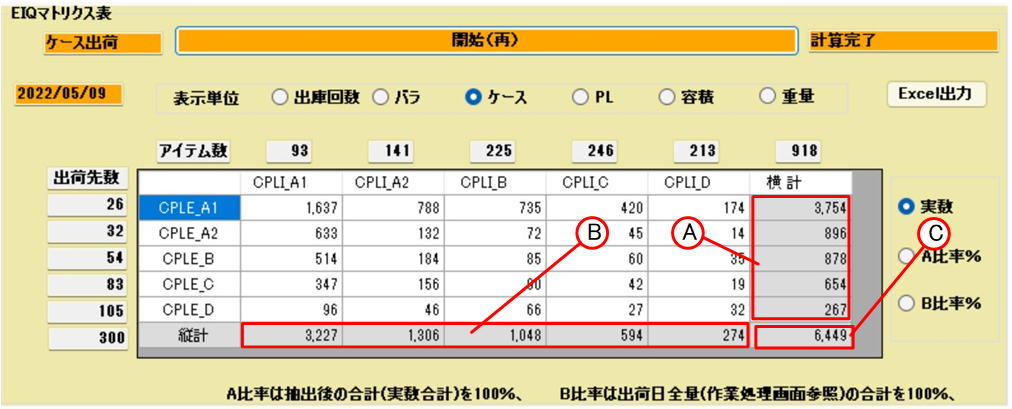
The EIQ Matrix Table can display data matching specific extraction conditions by designating those conditions.

When looking at the aggregation table, it is often confusing to distinguish between A1 rank of case shipping items, A1 rank of case shipping destinations, A1 rank of piece shipping items, A1 rank of piece shipping destinations, etc. To eliminate this confusion, we have devised a way to identify the contents of the table at a glance by looking at the rank symbol.

The meaning of the rank symbol "CKeE_A1" (CケE_A1) is: 1st character, "C" for Case shipping and "B" for Piece (Bara) shipping. 2nd character, the data item used for rank division: "Row" (行) for number of rows (picking frequency), "Piece" (バ) for piece quantity, "Ke" (ケ) for case conversion, "PL" for pallet conversion, "Vol" (容) for volume conversion, "Wgt" (重) for weight conversion.

3rd character, "E" for shipping destination rank, "I" for item rank. 4th character, "A1" for A1 rank, "A2" for A2 rank, "B" for B rank, "C" for C rank, "D" for D rank. Therefore, the rank symbol "CKeEA1" represents case shipping, ranking based on case conversion, and the A1 rank of the shipping destination.

Observation: When cropping the EIQ Matrix Table and pasting it into another document, be careful to explicitly note the "Shipping Method (Case Shipping)", "Shipping Date (2022/05/09)", and "Display Unit (Case)" above the cropped table, otherwise it will become unclear what the aggregation represents.

Item 5: Data Analysis Aggregation

The initial screen of Tera Calculation 1.

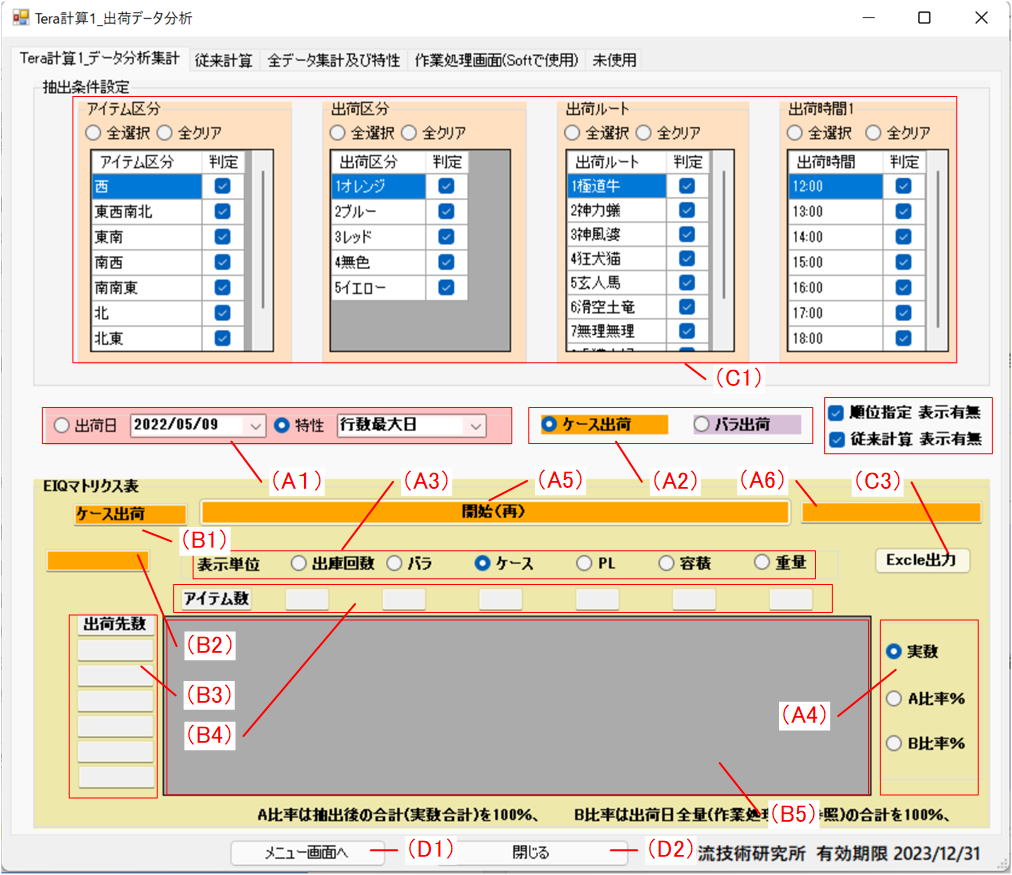
(A1) Clicking the Shipping Date radio button aggregates by specifying a shipping date. Clicking the Characteristic radio button allows you to select characteristics such as max row day, max case shipping day, and max piece shipping day.

(A2) Select either Case Shipping or Piece Shipping via the radio buttons.

(A3) Select one of the 6 Display Unit radio buttons, such as picking frequency, pieces, etc.

(A4) Select either Real Number or Ratio % via the radio buttons. After making selections in (A1) to (A4), click the Start button (A5) to begin processing.

(A6) The processing status is displayed in the text box.

After calculation processing, the output category (case/piece) is displayed in (B1), the shipping date in (B2), the number of shipping destinations in (B3), the number of items in (B4), and the EIQ Matrix Table is output to the data grid view (table) in (B5).

The matrix table can display real numbers and ratio %. Ratio A % displays the ratio of each rank by setting the post-extraction total (real number total) as 100%, and Ratio B % sets the total of the entire shipping day volume as 100%.

(C1) Allows you to select targets using checkboxes from 4 shipping condition items in the shipping data (multiple selections possible). Data (shipping data records) of items without a checkbox mark are excluded when calculating the EIQ Matrix Table.

(C3) The EXCEL output button exports the EIQ Matrix Table to Excel.

---

Section 2: Logistics Equipment Allocation

This section explains "Allocation of Logistics Equipment and Confirmation of Physical Volume Flow", which is the step following shipping data analysis.

This is the process of calculating the required floor area and processing capacity of the equipment by assigning specific logistics equipment to the physical volume of each block derived from the EIQ Matrix calculation.

1. Procedure for Allocating Logistics Equipment

On the Tera Calculation 1 screen, set the optimal equipment according to the item rank (fluidity).

• Specifying Equipment: From the selection field on the screen, specify equipment such as automated warehouses (PL_AS/RS), motorized racks, fixed racks, sorting machines, etc.
• Allocating to Cells: By clicking the cell corresponding to each item rank in the EIQ Matrix Table, the equipment is linked.
• Initial Settings: At startup, standard equipment is already allocated based on the "Tera Settings", so make changes as necessary.

2. Visual Confirmation via Physical Volume Flowchart

You can confirm at a glance which equipment how much physical volume passes through, from receiving to inventory to shipping.

• Receiving and Storage:
  • PL Single-Load Receiving: Items received by the pallet are stored directly in the empty racks of the equipment.
  • Case Receiving: It is assumed that items received by the case undergo "mixed-load storage," where multiple items are placed on a single pallet.
• Display of Inventory Data: Displays numerical values such as the number of items, piece quantity, case conversion, and PL conversion. Pallet load configurations can also be displayed, categorized from single-load up to a maximum of 8 mixed-loads.
• Movement to the Shipping Operation Area: Shows which operational equipment (flow racks, medium-duty racks, sorting machines, etc.) the products retrieved from the inventory equipment pass through before being shipped. The display unit synchronizes in real-time with the selection made in the "Shipping Volume" column (PL, cases, etc.).

3. How to Read the Table (Example)

Specific aggregation results are read as follows.

Item 1: Logistics Equipment Allocation

By allocating logistics equipment to the EIQ Matrix Table, the required area and necessary processing capacity of the logistics equipment can be calculated.

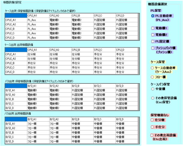
1. Specify the equipment in the Logistics Equipment Facility Selection column (figure on the left).

2. By clicking a cell in the table below, the equipment is allocated to the respective item rank.

(Since equipment is already allocated by the Tera Settings at startup, this becomes a task of modifying the equipment.)

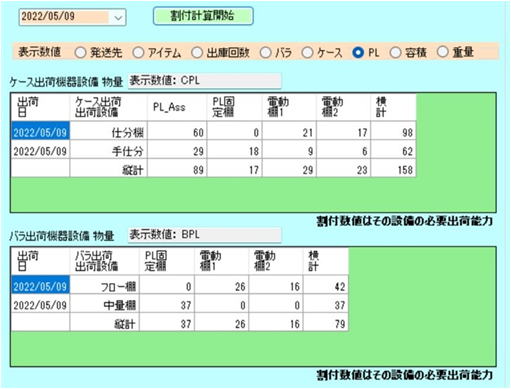
The table is read as: A total of 89 PLs are retrieved from PL_ASS, and transported as 60 PLs to the sorting machine and 29 PLs to manual sorting.

Item 2: Confirmation via Flowchart

Displays a comprehensive overview of physical volume from receiving, to inventory, and finally to shipping.

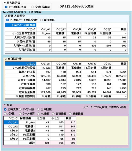
Select case unit shipping or piece unit shipping. It shows which logistics equipment facility the receiving goes to. It displays the number of items and the storage unit (PL unit, case unit). Displaying it in volume conversion has also been made possible.

Displays the number of items and piece quantity stored in the inventory equipment, as well as conversion values converting the piece quantity into case conversions, PL conversions, etc. Displays stored PL load configurations from single-load up to 8 mixed-loads.

Indicates whether stored products are shipped via equipment facilities in the shipping operation area, denoting the number of shipping destinations, number of items, picking frequency, and piece quantity. Conversions of piece quantities are also displayed.

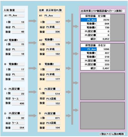
When the received product is a PL single-load (1 item loaded on a pallet), it can be imagined that it is stored in PL units in the empty racks of the equipment facility. When the received products are in cases, they undergo mixed-load storage (multiple items loaded on a pallet).

The physical volume heading towards the equipment facilities in the shipping operation area changes its display unit synchronously with the selection in the "Shipping Volume" column in the diagram above.

---

Section 3: Relationship Between Shipping Data, Receiving, and Inventory

This section explains the fundamental concepts and calculation logic for deriving inventory and receiving volumes from shipping data.

1. Basic Relationship of Shipping, Receiving, and Inventory

The flow of physical volume in a distribution center is expressed by the following formula.

• Characteristics of Shipping: Based on customer orders, so the center side cannot control the quantity or delivery date.
• Characteristics of Receiving: An operation to secure inventory, allowing the center side to dictate quantities and delivery dates to suppliers.
• Purpose of Inventory: To secure a quantity that prevents stockouts against daily fluctuating shipping volumes, while simultaneously compressing it as much as possible to reduce costs.

2. Logic for Estimating Inventory Quantity (Storage Quantity)

Tera Calculation calculates the inventory volume during stable operation using the following formulas.

• Daily Shipping Volume: Uses the average value of all shipping data.
• Concept of Inventory Days: Managed based on "Average Shipping Volume × Number of Days."
• Application to Actual Practice: Since this calculated value represents a theoretical average storage volume, if practical leeway is required, add an "allowance rate" to adjust it after calculation.
• Supplement: The "reorder point" is not considered in the calculation of inventory volume. The reorder point is merely an indicator of the ordering timing to guarantee inventory until the next receiving.

3. Handling of "Dead Stock" Not Appearing in Shipping Data

Not all inventory items move within the shipping data period subjected to analysis. Low-fluidity items, in particular, may have zero shipping records.

• Addition to Ranks: In Tera Calculation, inventory items that do not appear in the shipping data (no allocations) are added to the D Rank of piece shipping during inventory and receiving calculations.
• Limitation of Target: This addition process is performed only for piece shipping items, and is not applied to case shipping items.

With these steps, preparations are complete to estimate the overall volume of the entire center, including not just "moving physical volume" but also "dormant inventory" derived from the shipping data.

Item 1: Shipping, Receiving, and Inventory

Receiving, shipping, and inventory can be represented by the relationship: "Cumulative Receiving - Cumulative Shipping = Inventory".

Because shipping consists of orders from customers, the distribution center cannot arbitrarily increase or decrease shipping volumes or alter delivery dates. Inventory must be secured in quantities that prevent stockouts against daily fluctuating shipping volumes. At the same time, due to the need for inventory cost reduction and scale constraints of the distribution center, the inventory quantity should be kept as small as possible.

Inventory is managed for each item using the calculation: Average Shipping Volume * Number of Days = Maximum Inventory Quantity.

Receiving is the operation of placing orders with suppliers and having them delivered to the distribution center to secure inventory. While the distribution center cannot change shipping dates or volumes, it can instruct the quantities and delivery dates for receiving (Is this really true in practice?). For methods of calculating receiving and inventory from shipping data, refer to Tera Calculation's Inventory Volume Estimation and Receiving Volume Estimation.

Item 2: Inventory Not Included in Shipping Data (Unshipped Items)

There are inventory items not included in the entirety of the shipping data (spanning multiple shipping days).

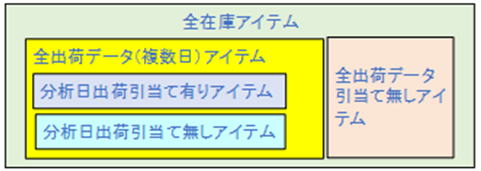
While high-fluidity items are included in the shipping data, low-fluidity items might not be.

In Tera Calculation, items with no allocations in the entire shipping data are added to the D rank when performing inventory and receiving calculations.

Note: They are added to the D rank of piece shipping items, but are not added to case shipping.

Item 3: Calculation of Inventory Quantity (Storage Quantity)

There are inventory items not included in the total shipping data (across multiple shipping days).

Inventory can be expressed by the relationship: "Cumulative Receiving - Cumulative Shipping = Inventory". Because shipping comprises customer orders, the distribution center cannot alter shipping volumes or delivery dates for its own convenience. Inventory must secure enough quantity to avoid stockouts in response to daily fluctuating shipping volumes.

On the other hand, due to inventory cost reduction and space limitations of the distribution center, it is desirable to keep inventory levels as low as possible. Inventory is managed for each item via the calculation: Average Shipping Volume * Number of Days = Maximum Inventory Quantity.

Receiving is the business of ordering from suppliers and having goods delivered to the distribution center to secure inventory volumes. While shipping dates and volumes cannot be altered for shipping, for receiving, the distribution center can dictate quantities and delivery dates. Based on these premises, Tera Calculation estimates inventory volumes and receiving volumes from shipping data.

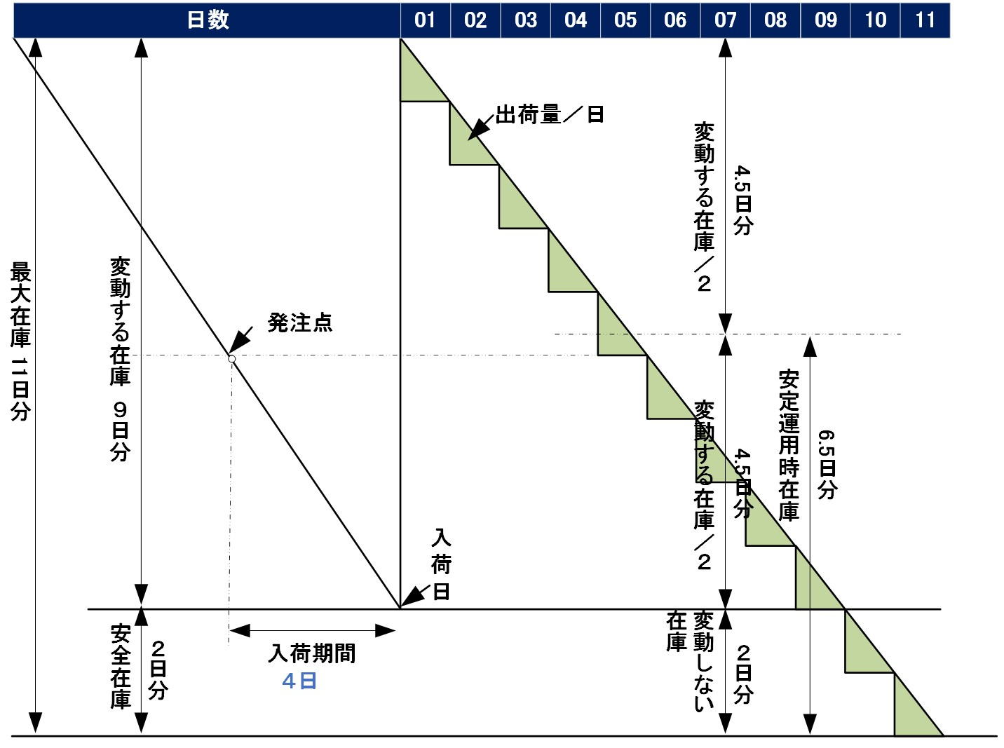
The Shipping Volume / Day uses the average value of all data.

The method Tera Calculation uses to find the inventory storage volume is: Stable Operation Inventory (Storage Volume) = Safety Stock + (Variable Inventory / 2), where Variable Inventory = Maximum Inventory - Safety Stock (refer to Section 2).

For example, suppose there are 18 items with a maximum inventory of 11 days, safety stock of 2 days, and variable inventory of 9 days. If you receive 3 of these items every day, the fluctuating inventory storage volume = (Variable Inventory / 2).

If calculating the stable operation inventory (storage volume) seems unrealistic in actual practice, you can simply add an allowance rate after performing the above calculation.

Note: The reorder point has no bearing on calculating physical inventory volumes; the reorder point is the inventory level that triggers a purchase order, timed to guarantee inventory for the period from placing the order until the goods are received.

---

Section 4: Inventory and Receiving Calculation

This section explains the fundamental concepts and calculation logic for deriving inventory and receiving volumes from shipping data.

1. Basic Relationship of Shipping, Receiving, and Inventory

The flow of physical volume in a distribution center is expressed by the following formula.

• Characteristics of Shipping: Based on customer orders, so the center side cannot control the quantity or delivery date.
• Characteristics of Receiving: An operation to secure inventory, allowing the center side to dictate quantities and delivery dates to suppliers.
• Purpose of Inventory: To secure a quantity that prevents stockouts against daily fluctuating shipping volumes, while simultaneously compressing it as much as possible to reduce costs.

2. Logic for Estimating Inventory Quantity (Storage Quantity)

Tera Calculation calculates the inventory volume during stable operation using the following formulas.

• Daily Shipping Volume: Uses the average value of all shipping data.
• Concept of Inventory Days: Managed based on "Average Shipping Volume × Number of Days."
• Application to Actual Practice: Since this calculated value represents a theoretical average storage volume, if practical leeway is required, add an "allowance rate" to adjust it after calculation.
• Supplement: The "reorder point" is not considered in the calculation of inventory volume. The reorder point is merely an indicator of the ordering timing to guarantee inventory until the next receiving.

3. Handling of "Dead Stock" Not Appearing in Shipping Data

Not all inventory items move within the shipping data period subjected to analysis. Low-fluidity items, in particular, may have zero shipping records.

• Addition to Ranks: In Tera Calculation, inventory items that do not appear in the shipping data (no allocations) are added to the D Rank of piece shipping during inventory and receiving calculations.
• Limitation of Target: This addition process is performed only for piece shipping items, and is not applied to case shipping items.

With these steps, preparations are complete to estimate the overall volume of the entire center, including not just "moving physical volume" but also "dormant inventory" derived from the shipping data.

Item 1: Inventory and Receiving Calculation Screen

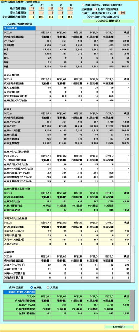
1. Input the Maximum Inventory Days and Safety Stock Days by rank.

2. Input the number of inventory items missing from the shipping data.

3. Calculate and output the average daily shipping volume, which serves as the basis for calculation.

4. Calculate the stable operation inventory days. Stable Operation Inventory (Storage Volume) = Safety Stock + (Variable Inventory / 2), where Variable Inventory = Maximum Inventory - Safety Stock (refer to Section 2).

5. Calculate the inventory volume during stable operation. Inventory Volume = Daily Shipping Volume * Stable Operation Inventory Days.

6. Calculate the inventory volume per item. Inventory Quantity per Item = Inventory Volume / Number of Items.

7. Determination of required pallet conversion numbers and single/mixed loads.

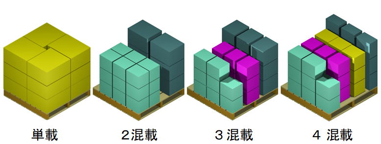
8. Calculation of number of receiving items and physical volume. Number of receiving items = Number of inventory items / Receiving cycle; Receiving Volume = Shipping Volume; Calculate Receiving Volume (for checking).

Clicking the Inventory Volume radio button displays the inventory volume, while clicking the Receiving Volume radio button displays the receiving volume.

9. Clicking the Excel button saves the inventory/receiving data to Excel.

The above explains piece shipping as an example; case shipping undergoes the same calculations. Note: Inventory not included in shipping is incorporated into piece shipping, whereas for case shipping, inventory missing from the shipping data is treated as 0.