Chapter 7: Tera Calculation Reference[cite: 13]
Section 1: EIQ Analysis[cite: 13]
What is EIQ Analysis?[cite: 13]
EIQ analysis is a method of analyzing the correlation between E (Entry: Destination), I (Item: Product), and Q (Quantity: Amount) from shipping data.[cite: 13] Its origins lie in the "seeding chart" created during "seeding work (piece picking)" that has long been practiced at logistics sites.[cite: 13]
Tera Calculation is based on the concept of "SEIQ", which adds product dimensional elements to this EIQ analysis, materializing conversions into practical units such as cases, pallets, volume, and weight.[cite: 13]
Main Analysis Outputs[cite: 13]
1. EIQ Table (Seeding Chart)[cite: 13]
A massive matrix table with items placed on the vertical axis and destinations on the horizontal axis.[cite: 13]
- Characteristics: Displays items sorted in descending order of shipping quantity.[cite: 13]
- Example: At a scale of 430 destinations × 1,984 items, for instance, the sheer volume of data is too enormous for the human eye to process at once.[cite: 13]
- Analysis Hints: If there are blanks among the top destinations, one can read a tendency of operational strategies dispersing shipments to specific days (e.g., handling only urgent shipments and suspending normal shipments).[cite: 13]
2. EIQ Scatter Plot[cite: 13]
This plot represents each cell (1 square) of the EIQ table as a dot depending on the presence or absence of a shipping record, visualizing the entire shipping data on a single screen.[cite: 13]
- Role: It is suitable for intuitively grasping the overall distribution tendency of the shipping data, but it is difficult to read detailed volumes (Q) from it.[cite: 13]
3. EIQ Matrix Table[cite: 13]
A table aggregated by dividing the EIQ table into a total of 25 blocks: "5 item blocks × 5 destination blocks."[cite: 13]
- Practical Advantages: It is a very easy-to-handle classification when considering the selection of logistics equipment and the allocation of facilities.[cite: 13]
- Flexible Calculation: It can display values converted not only into quantities, but also into units like number of cases, number of pallets, and volume.[cite: 13]
- Rankey Ratio: Through Tera Settings, the volume ratio (rankey ratio) of each block can be defined, setting the total at 100%, and these ratios can also be changed during data processing.[cite: 13]
Item 1: Creation of the EIQ Table[cite: 13]
EIQ Table Creation Screen[cite: 13]
The table displays data for the shipping date 2022/05/09, where items are sorted in descending order of piece count across all shipping data.[cite: 13]
Because destination ranks 1 and 2 were not shipped, they are left blank; scrolling will reveal the figures for all 438 destinations.[cite: 13]
Since there are 1,984 items, it is divided into 66 pages for display in consideration of the display range and the processing speed due to PC load.[cite: 13]
The size of this table is 430 rows * 1,984 columns, which as-is cannot be read by the human eye.[cite: 13]
Observations:[cite: 13]
In the table above, destinations 1 and 2 are blank. This means no shipments were made to the top 1 and 2 destinations. Perhaps there are urgent shipment items among the lower-ranked items, but it was a day off for regular shipping.[cite: 13]
Such operational strategies to intentionally disperse shipping dates are found in many distribution centers.[cite: 13]
Item 2: Creation of the EIQ Scatter Plot[cite: 13]
The EIQ scatter plot is a chart that represents 1 square (cell) of the EIQ table as a dot, displaying the entire shipping data on a single screen.[cite: 13]
EIQ Scatter Plot[cite: 13]
The chart is a scatter plot where cells with shipments are represented by dots to show the entire EIQ table.[cite: 13]
Unfortunately, while the overall trend can be seen, it is impossible to determine the volume.[cite: 13]
Item 3: Creation of the EIQ Matrix Table[cite: 13]
The EIQ Matrix Table is created by dividing the EIQ table into 5 item blocks * 5 destination blocks = 25 blocks and aggregating the data.[cite: 13]
From experience, this is considered a convenient number of block divisions when allocating equipment and facilities during system design.[cite: 13]
This table can calculate figures converted into cases, PLs, or volume as necessary.[cite: 13]
It is displayed alongside the conventional calculation, so please learn by comparing it with the conventional calculation method.[cite: 13]
EIQ Matrix Table[cite: 13]
The table shows that 1,099 records (rows) were shipped in the Case_I_A1 block, which has 132 items; within this, 488 rows were shipped to the top 21 destinations in the Case_E_A1 block,[cite: 13]
and 185 rows were shipped in the Case_I_A2 block, etc., totaling 1,009 rows (300 destinations) shipped in the Case_I_A1 block.[cite: 13]
Observations[cite: 13]
In the EIQ Matrix Table, under Tera Settings, volume is assigned to each block as a rankey ratio (%) based on a total of 100%, as shown in the table below.[cite: 13]
For information on rankeys, please refer to "Chapter 2: Tera Calculation 0_Shipping Data Processing."[cite: 13]
The ratios for each block can be changed by modifying the Tera Settings during Tera Calculation 0_Data Processing.[cite: 13]
The rank classification is performed by analyzing and aggregating the entire shipping data. An extracted EIQ matrix aggregation specifying a shipping date will result in slight ratio deviations.[cite: 13]
Section 2: Conventional Calculation[cite: 13]
ABC Analysis in Tera Calculation (Conventional Calculation)[cite: 13]
A general ABC analysis sorts shipping data from high liquidity to low liquidity and divides it into 3 segments (A, B, C) based on cumulative ratios. In contrast, Tera Calculation performs aggregation by dividing it into 5 blocks (ranks) to provide more flexibility in practical logistics equipment selection.[cite: 13] This is defined as "Conventional Calculation," and is utilized as a basis for system design while comparing it with the results of EIQ analysis.[cite: 13]
1. Overall Data Aggregation and Addition of Items[cite: 13]
We aggregate practical indicators that are not included in the shipping data itself to grasp the overall picture of the center.[cite: 13]
- Added Conversion Items: Case conversion, PL (pallet) conversion, volume conversion, and weight conversion.[cite: 13]
- Estimation of Case Dimensions: Even if the shipping data lacks case dimensions, they are estimated from case volume data by visualizing dimensions with a ratio of "length 5 : width 4 : height 3".[cite: 13]
- Aggregation Characteristics: It visualizes the characteristics of all data, such as case quantities varying widely from 1 to 120.[cite: 13]
2. Aggregation by Shipping Unit and Rank[cite: 13]
In logistics system design, the classification of "case shipping" and "piece shipping" is extremely important because their storage and operational methods differ.[cite: 13]
Classification by Shipping Unit[cite: 13]
- Case Shipping: Shipping records conducted in case units.[cite: 13]
- Piece Shipping: Shipping records conducted in piece units.[cite: 13]
- Case/Piece Shipping: A case where a single record is shipped as, for example, "1 case + 3 pieces." Computationally, this is incorporated into the respective rank calculations as 1 case shipment and 1 piece shipment.[cite: 13]
Equipment Allocation via Aggregation by Rank[cite: 13]
Subdividing ABC analysis into 5 blocks creates flexibility in the allocation of facilities and equipment.[cite: 13]
- Example: It makes specific considerations easier, such as "combining ranks A1 and A2 for electric racks" or "using fixed racks for ranks A2 and B."[cite: 13]
- Consistency: This aggregation result is designed to match the classifications of the EIQ Matrix Table.[cite: 13]
3. Utilization of Pareto Charts (ABC Analysis)[cite: 13]
It is also possible to display, for reference, a Pareto chart (ABC distribution) representing each item by monetary value or volume.[cite: 13]
- Observations: Value-based analysis is useful for purchasing or sales departments; however, in logistics system design (equipment selection), volume-based aggregation by rank serves as a stronger basis for design.[cite: 13]
Item 1: Overall Data Aggregation[cite: 13]
Conventional Calculation Screen[cite: 13]
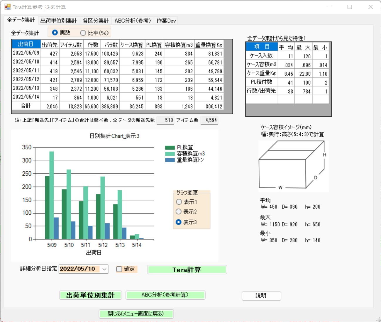
The "Shipping Data Aggregation" table on the left is an aggregation of all shipping data by item category, to which case conversion, PL conversion, volume conversion, and weight conversion—items not found in the original shipping data—have been added.[cite: 13]
The "Ratio %" radio button represents the ratio of each shipping day when the total shipping data is set as 100%.[cite: 13]
The total values for destinations and items in this shipping data are cumulative figures that overlap and are shipped on a daily basis.[cite: 13]
The shipping data contains 518 destinations and 4,594 items (as noted in the table).[cite: 13]
The "Graph" is for the shipping date 2022/05/10.[cite: 13]
Display 1 shows destinations, items, and row counts.[cite: 13]
Display 2 shows piece counts and case conversions.[cite: 13]
Display 3 shows PL conversions, volume conversions, and weight conversions.[cite: 13]
As a "characteristic seen from the overall data aggregation,"[cite: 13]
case quantities are extremely diverse, ranging from 1 to 120.[cite: 13]
While the shipping data contains case volume data, it lacks the concept of case dimensions.[cite: 13]
The "Case Volume Image" visualizes case dimensions with a ratio of length 5, width 4, and height 3.[cite: 13]
Calculating the case volume implies that case dimension data exists as a separate dataset; thus, by linking the case dimension data with the shipping data, individual item dimensions can be understood. Tera Calculation estimates the case dimensions under the assumption that case dimension data is not on hand.[cite: 13]
Case shipping and piece shipping have different storage and operational methods.[cite: 13]
In the overall data aggregation screen above, case shipping and piece shipping are not separated, so equipment allocation cannot be performed. This serves as reference data for system design.[cite: 13]
Item 2: Aggregation by Shipping Unit[cite: 13]
Aggregation by Shipping Unit Screen[cite: 13]
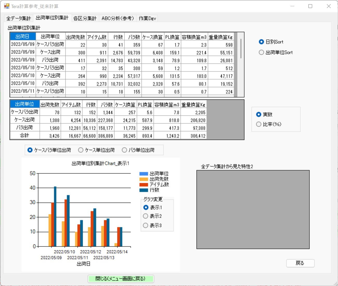
The way to read the table is the same as the conventional calculation screen.[cite: 13]
Aggregation is performed separately for case shipping and piece shipping.[cite: 13]
Normally, a record indicating case shipping (a row in the shipping data) involves shipping in case units. The same applies to piece shipping.[cite: 13]
Rarely, there are shipments where 1 record involves 1 case plus an additional 3 pieces. Mixed case/piece shipping refers to this type of shipment.[cite: 13]
This mixed case/piece shipping is treated as 2 shipments for 1 record—1 case shipment and 1 piece shipment—and is incorporated into the case shipping and piece shipping during rank calculation.[cite: 13]
Note:[cite: 13]
The figures for mixed case/piece shipping will not appear after the rank aggregation.[cite: 13]
In the explanation of the overall data aggregation, it was stated that "case shipping and piece shipping have different storage and operational methods." It is also true that "case shipping and piece shipping differ in storage and operational methods even based on volume."[cite: 13]
Equipment allocation cannot be performed using the classified aggregation of case shipping and piece shipping. This serves as reference data for system design.[cite: 13]
Item 3: Aggregation by Rank[cite: 13]
Conventional Calculation (Applied ABC Analysis)[cite: 13]
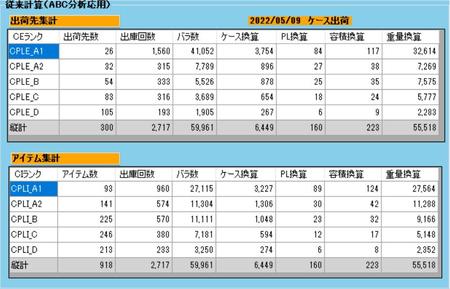
The table on the left is the table displayed in "Tera Calculation 1_Shipping Data Analysis."[cite: 13]
This table extracts and aggregates case shipping; a similar aggregation is possible for piece shipping.[cite: 13]
ABC analysis is aggregated into 5 divisions rather than 3.[cite: 13]
It is possible to verify how much of each rank's items are shipped, including not only piece counts but also converted values.[cite: 13]
Because this aggregation uses the same classifications as the EIQ Matrix Table, the aggregation results will match the EIQ Matrix Table.[cite: 13]
Because the table above separates case shipping and piece shipping and performs ranking, equipment and facilities can be easily allocated.[cite: 13]
The allocation of storage facilities uses the average of all data (refer to Chapter 3: Tera Calculation 1_Shipping Data Analysis, Section 2: Allocation of Equipment and Facilities) and utilizes item aggregation.[cite: 13]
By dividing into 5 blocks, flexibility in allocation is achieved, such as combining Case_PL_I_A1 and Case_PL_I_A2 for electric racks, or making Case_PL_I_A2 and Case_PL_I_B fixed racks.[cite: 13]
Item 4: ABC Analysis (Pareto Chart)[cite: 13]
ABC Analysis (Reference) Screen[cite: 13]
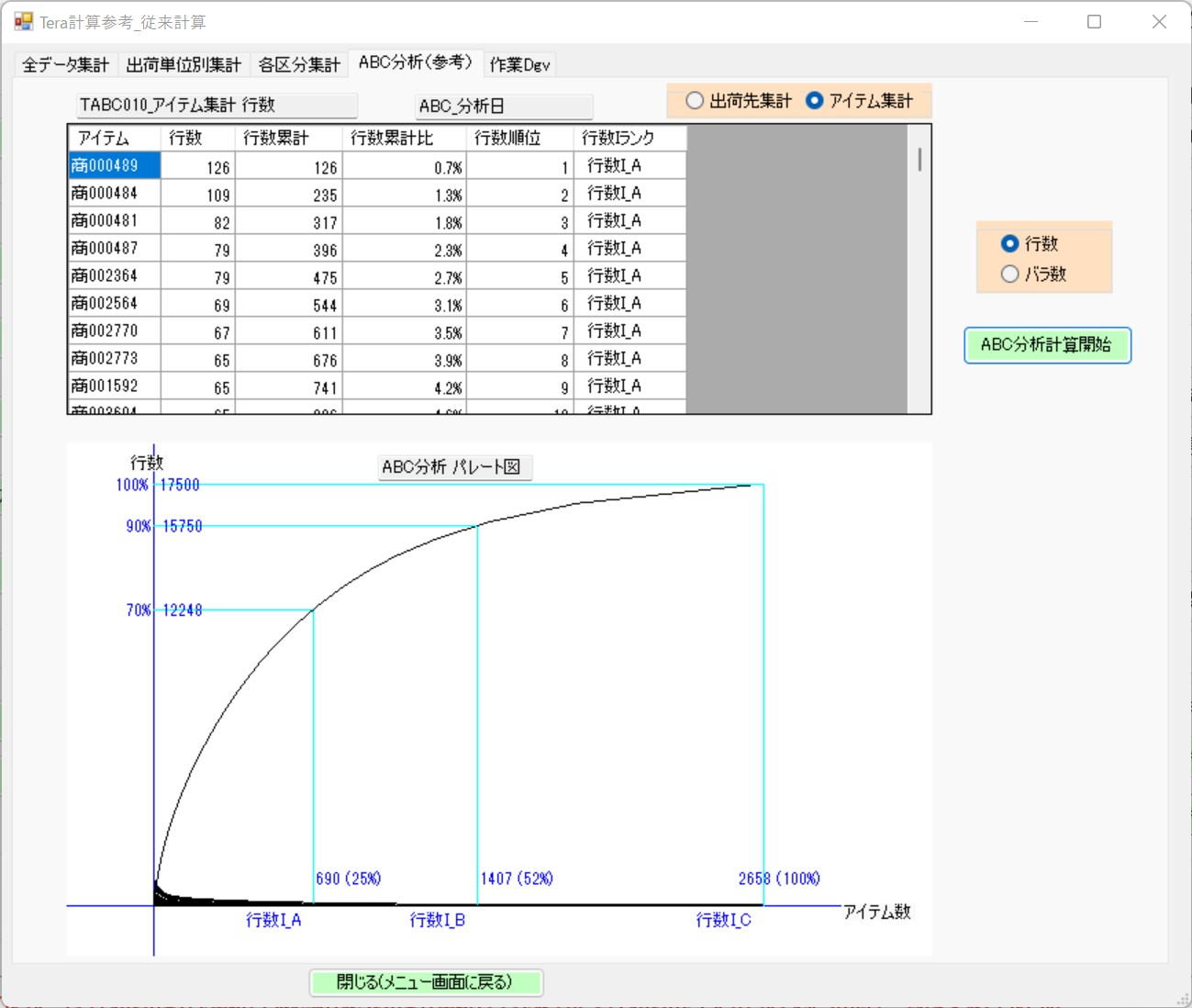
The table on the left displays ABC analysis for reference.[cite: 13]
The table is a sort ranking table of item aggregation intended for displaying a Pareto chart.[cite: 13]
Case shipping and piece shipping are aggregated separately.[cite: 13]
There are cases where the ABC distribution is expressed using the monetary value of each item. While this may be a valuable aggregation for purchasing and sales departments, it serves merely as reference material in system design and provides a weak basis for determining the system.[cite: 13]